

To complete the servicing, the file must be at Finance Submission Stage.
In designing any banking tool – it is firstly important to acknowledge that there is no one “right” approach to assess the capacity of the borrower. Both the nature of the assets being funded, and the type of lender you are approaching, will drive the specific measurements used for servicing.
The approach of CLE is to start with a consistent and readily understood approach. This begins with normalising the Operating Profit before Taxation as per the example below:
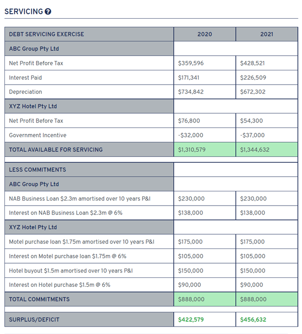
As a starting point, regardless of the method applied by the lender, identification of whether there is a surplus remaining after all commitments is important.
It is important to include in this process a review of the Profit & Loss to adjust for any abnormal or non-recurring incomes/expenses. These should be adjusted for, and Total Available for Servicing will be calculated.
In smaller SME’s, adjustments may include an assessment of the owners’ salary. It is important the owner personal exertion contributed to the business is costed at a market rate.
COMPONENTS OF SERVICING
The components of loan serviceability can include many measures – explained by applying the data in the example above.
Interest Cover Ratio (“ICR”)
A measure of how easily a business can pay interest on its outstanding debt. Using the example this is calculated as:
Total EBIT ($1,344,632) / Total Interest ($333,000) = 4.03
When a trading company's interest coverage ratio is 2.0 or lower, its sustained ability to meet interest commitments may be questionable, especially if there is uncertainty around the reliability of the future income.
ICR is also commonly applied for assessing consistent yield assets. For example, rental income on a commercial investment property. Expect ICR’s to be lower in these examples where there is no trading income to support servicing.
Debt Service Ratio (“DSR”)
A measure of how easily a business can pay total debt repayments on its outstanding debt. Using the example this is calculated as:
Total EBIT ($1,344,632) / Total Debt Commitments ($888,000) = 1.51
Where this ratio is 1.0 or lower, cash flow will be negative! So how close it goes to 1.0 times depends on the quality and certainty of the income of the business.
DSR can be a more relevant measure of liquidity, unlike ICR it includes the actual cash commitment to reducing debt. Where strong amortisation is needed, the gap between DSR and ICR can be very wide.
Payback (Debt) Ratio
A measure of how quickly total debt can be repaid out of EBIT and cash reserves. Using the example this is calculated as:
Total Debt ($5,550,000) - Cash ($120,000) / Total EBIT ($1,344,632) = 4.04
The greater the uncertainty around future earnings, the more quickly the business may want to retire debt. This is mitigated too by the price of the debt, where there may be great returns from deploying cash elsewhere.
As relevant as the actual Payback Ratio result is the variation from period to period.
Multiple of Earnings
A less commonly communicated but valid test of borrowing capacity is to apply a multiple limit to the adjusted EBITDA.
This has become increasingly popular in assessing borrowing capacity for professional service firms. Using the example this is calculated as:
Total EBIT ($1,344,632) x Maximum Multiple of 3.0 = $4,033,896 (Indicative Borrowing Capacity).
Usually an appropriate method where consistency of EBITDA is evident.